PROBLEM LINK:
Author: Malvika Raj Joshi
Tester: Roman Furko
Translators: Vasya Antoniuk (Russian), Team VNOI (Vietnamese) and Hu Zecong (Mandarin)
Editorialist: Kevin Atienza
DIFFICULTY:
Hard
PREREQUISITES:
Centroid decomposition, segment tree, disjoint set union, power-of-two pointers
PROBLEM:
There are N nodes forming a tree. Each node contains a tulip, and each edge has a given length. If a tulip is picked, a new one will grow in the same spot if it is left undisturbed for X contiguous days.
On day d_j, Cherry visits all node reachable from u_j with edges of length \le k_j. She will pick all the tulips she can find. On day d_1, all nodes have tulips.
For each of the Q days Cherry does this, print the number of tulips she gets.
QUICK EXPLANATION:
-
Construct the “reachability tree” of the given tree. We define the reachability tree as a rooted binary tree with 2N-1 nodes such that each leaf represents a node in the original tree, and each internal node represents a set of nodes in the original tree that are reachable from each other using edges up to a certain length. In other words, each internal node is associated with some value, say k, such that the leaves under it represent a maximal set of nodes in the original tree that are reachable from each other using edges of length \le k. This tree can be constructed in O(N \log N) time.
-
Compute the preorder traversal of the leaves of this tree. Now, the nodes in the original tree in this traversal has the property that any visitation by Cherry always affects consecutive nodes in the traversal, making it amenable to range query optimizations.
-
Construct a segment tree on top of this traversal that can support the following operations:
- initialize: Initialize all values to 0.
- update: Given a subrange, increase/decrease it by a given amount.
- query: Given a subrange, how many values in it are equal to 0?
The structure may assume that all values will stay nonnegative.
-
For every visitation (d_j,u_j,k_j), first find in the preorder traversal the range [l,r] of nodes reachable from u_j using edges of length \le k_j. (This can be done in O(\log N) time using power-of-two pointers.) Next, print the number of values in the segment tree in the subrange [l,r] equal to 0. Next, increase all elements in the subrange [l,r] by 1. Finally, add a future decrement operation that will decrease all elements in the subrange [l,r] by 1 on day d_j+X. (You will need to perform these decrement operations before processing visitations on or after that day. You can keep track of these future decrements using a queue, because d_j+X is increasing.)
(Note: there are many other approaches as well)
EXPLANATION:
Traversing edges up to a given length
Each visitation has a starting node u and a number k, and performs some operations across all nodes that are reachable from u using edges with weights \le k. We will use the notation R(u,k) to denote the set of nodes reachable from u using edge with weights \le k. Clearly, we can’t iterate through all nodes of R(u,k) for every visitation because that would be slow. So to progress, we must study the R(u,k) sets more closely.
Let’s consider a fixed u, and a varying k. k starts at 0 and continuously increases up to \infty. Let’s see what happens to R(u,k) while this happens. In the beginning (k = 0), no edges are usable, so R(u,k) is simply \{u\}. As we increase k however, more and more edges become usable, giving us access to more nodes, so R(u,k) possibly increases in size. Eventually, k will surpass the largest edge weight in the tree, and R(u,k) becomes the set of all N nodes.
There are two things that we learn from this process:
- As we increase k, \left|R(u,k)\right| never decreases in size.
- Not only that, but we can also say that for k < k', R(u,k) \subset R(u,k')! In other words, once a node becomes reachable from u, it becomes reachable forever.
These are certainly nice facts. Unfortunately these don’t give us the full picture. So let’s look at the full picture. Instead of focusing on a fixed node u, we will focus on all N nodes. Specifically, we will focus on R(u,k) for all nodes u (not just a fixed u), as we increase k.
As before, in the beginning, no edge is usable, so R(u,k) = \{ u \} for all nodes u. Now, as we increase k, one by one each edge becomes usable, effectively uniting the set of reachable nodes it connects. Specifically, once the edge (u,v) becomes usable, R(u,k) and R(v,k) unite and become equal. This happens one by one for each edge, until finally k passes the largest edge weight, and all sets R(u,k) unite into a single set containing all N nodes.
So, what did we learn from this experiment? We learned that the sets R(u,k) behave as if we’re doing union-find. Moreover, upon closer look, we can also see some sort of tree structure behind all this!
Let’s call this tree the reachability tree. We will define the reachability tree as a rooted binary tree with 2N-1 nodes such that:
- Each leaf represents a node in the original tree, and
- Each internal node represents a union operation during our experiment above.
We call this the “reachability tree” because each internal node represents some R(u,k) at some point during our experiment above. More specifically, each internal node is associated with some value, say k, such that its leaves constitute some R(u,k).
Let’s give an example. Consider the following tree:
<img src=“https://discuss.codechef.com/upfiles/1_11.png”, width=“100%”>
The reachability tree of this tree is the following:
<img src=“https://discuss.codechef.com/upfiles/2_8.png”, width=“100%”>
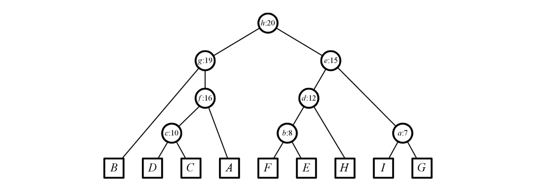
Note that the original nodes are leaves in this reachability tree. Also, every internal node represents some R(u,k). For example, node f represents the set R(A,16) = R(C,16) = R(D,16) = \{A, C, D\}.
The reachability tree has the following nice property:
Given any u, k, R(u,k) is always the set of leaves of some subtree in the reachability tree. (This includes any k, not just values associated with internal nodes.)
For example, suppose that in the tree above, we start at node F and traverse all edges with weight \le 14. Then R(F,14) = \{F, E, H\}, as shown in the following:
<img src=“https://discuss.codechef.com/upfiles/3_2.png”, width=“100%”>
True enough, these nodes can be found as leaves of some subtree in the reachability tree:
<img src=“https://discuss.codechef.com/upfiles/4_2.png”, width=“100%”>
This property of the reachability tree is very useful for us, as we intend to operate on R(u,k) sets many times. To see why it’s useful, note that when we perform a preorder traversal of the tree and collect the leaves during this traversal, the set of leaves of any subtree can be found in consecutive positions in the traversal. This allows us to turn any operation on the set R(u,k) into a range query! Thus, this tree can help us immensely if we can construct it.
Constructing the reachability tree
We can construct the reachability tree by remembering how we discovered it: by uniting sets together, starting from N sets to just one. This is very much like union-find, except that during every union, we also create a new node recording that union in the reachability tree.
That is the main idea of the construction. We’re building the tree from the ground up, starting from the leaves up until the root. We will maintain disjoint sets representing $R(u,k)$s. In addition, each disjoint set’s representative points to its current root node in the reachability tree.
- Initially, all N nodes are on separate sets, each pointing to a new node. These new nodes are the leaves of the reachability tree.
- Next, we iterate through all edges in increasing order of weight. For each edge (u,v) with weight k, we unite the sets containing u and v, and create a new node in the reachability tree whose children are the nodes being pointed at by u's and v's representatives.
- After iterating through all N-1 edges, we now have the reachability tree!
This runs in O(N \log N) time because we sorted the edges. Everything else runs asymptotically faster.
Performing queries
Next, we need to convert a query (d_j,u_j,k_j) into a range query, with the help of the reachability tree. We will assume that we’ve already performed the preorder traversal on the reachability tree, and collected all leaves in this traversal.
Our goal now is to find the relevant range of nodes [L_j,R_j] corresponding to the set R(u_j,k_j). There are two steps we need to take:
- Given u_j and k_j, find the subtree that contains all nodes of R(u_j,k_j) (and only those nodes). Let p be the root of this subtree.
- Given this subtree rooted at p, find the indices of the leftmost and rightmost leaves. (These indices are the L_j and R_j we are looking for.)
Let’s look at the first step. We need to find p. Surely, p is an ancestor of u_j in the reachability tree. More specifically, p is the highest ancestor of u_j whose associated value k is \le k_j. This gives us a way of computing p, but it’s slow (because the reachability tree can be highly imbalanced).
So how do we compute p quickly? It would be nice if we can binary search along all ancestors of u_j. But we can actually do that with the help of power-of-two pointers (also called jump pointers). The idea is, for each node in the reachability tree, to store all its ancestors at power-of-two heights, i.e. for every i \ge 0, we store its $2^i$th ancestor. This structure is usually used to compute certain ancestors of nodes quickly (and is also used in computing lowest common ancestors), but we can also use this structure to compute p quickly. The following pseudocode illustrates the idea:
// in this code, u.jump(i) is the 2^i'th ancestor of u
def find_p(u_j, k_j):
    if nodes[ROOT].k <= k_j:
        return ROOT

    i = 0
    while u.jump(i).k <= k_j:
        u = u.jump(i++)

    while i != 0:
    	i--
        if u.jump(i).k <= k_j:
            u = u.jump(i)

   return u
The first part simply checks if the root is already a valid p. Otherwise, the first while loop simply finds some ancestor that is not a valid p. The second while loop then finds the smallest ancestor that is not a valid p. So after that loop, the ancestor before that must be the p we are looking for!
Now, for the second part. Given a subtree rooted at p, what is the leftmost and rightmost leaf? This is actually easier: Simply precompute all leftmost and rightmost leaves using a single traversal and dynamic programming! The following recurrences can be used:
Now, we can convert (d_j,u_j,k_j) into a range query on the range [L_j,R_j]!
Range queries
Now that all queries are now range queries, let’s write the current version of the problem:
There are N nodes in a line. Each node contains a tulip. If a tulip is picked, a new one will grow in the same spot if it is left undisturbed for X contiguous days.
On day d_j, Cherry visits all nodes from L_j to R_j and picks all the tulips she can find. On day d_1, all nodes have tulips.
For each of the Q days Cherry does this, print the number of tulips she gets.
This sounds much doable because we’ve essentially gotten rid of the tree and replaced it with range queries. We’ve now essentially flattened the problem. All that remains is to find a way to perform the range queries efficiently!
The idea for our fast solution would be to create an array of N elements, [D_1, \ldots, D_N], where D_i represents the “disturbance” of the i th node. Here, we define the disturbance of a node as the number of times the node has been disturbed in the past X days. This way, a node has an available tulip if and only if its disturbance is 0. Initially of course, D_i = 0 for all i.
Now, when nodes L_j to R_j are visited on day d_j, these things happen:
- Count the number of available tulips in the range. Specifically, count the number of nodes in the range [L_j,R_j] with disturbance equal to 0.
- Disturb these nodes, i.e. increase the disturbance of all nodes from L_j to R_j by 1. However, we must remember to decrease them again after X days, i.e. on day d_j+X.
So all in all, three events happen for each visit (d_j,L_j,R_j):
- On day d_j, we count the number of i s in the range [L_j,R_j] where D_i = 0.
- On day d_j, we increase all disturbances in the range [L_j,R_j] by 1.
- On day d_j+X, we decrease all disturbances in the range [L_j,R_j] by -1.
Thus, to process all visitations, we just need to sort all the events across all visitations altogether. If multiple events happen on the same day, perform decrease operations before queries, and perform queries before increase operations.
But how do we handle range increases/decreases and range queries? At first glance, it seems hard to find any efficient segment tree solution, but things become much easier when you notice that disturbances never drop below 0. So if the disturbance 0 is present in the range at all, then it is surely the minimum disturbance in that range. Thus, to answer the range query “how many disturbances are equal to 0”, we can use the following more general range query:
- Given a subrange [L_j,R_j], what is the minimum disturbance in this range, and how many times does it appear?
To answer our original range query, we simply perform this new range query on the range and then check if the minimum disturbance is 0. If it is, then return the count, otherwise, simply return 0. ![]()
Thus, all we need to implement is a typical range minimum query structure with range updates, with a slight twist: we also need to count how many times the minimum appears. But our trusty segment tree with lazy propagation can do this job very efficiently! We just need to modify it slightly so that the count can also be returned. To do it, simply add this count in every node of the segment tree, and remember to update it during downward propagations, updates and queries!
For implementation details, see the tester’s or editorialist’s code.
Now, what is the time complexity? Clearly, O(\log N) time is needed for each query/update, so all events run in O(Q \log N) time. Initializing the segment tree requires O(N) time, and computing the sorted order of the events requires O(Q \log Q) time. By including the fact that the reachability tree is constructed in O(N \log N) time, the overall complexity becomes O((N+Q)\log N + Q\log Q).
We can actually remove the O(Q \log Q) bit by noticing that the visits are given in increasing order of d_j already. This means that the only out-of-order events are the decrease events, and even they are already given in increasing order (since d_j+X is increasing). Thus, all we need to do is to merge two sorted list of events together. The merge routine of merge sort does this job in O(Q) time. With this, the overall running time becomes just O((N+Q) \log N).
Time Complexity:
O((N+Q) \log N)