Problem Link
Author: Ivan Safonov
Tester: Hasan Jaddouh
Editorialist: Bhuvnesh Jain
Difficulty
MEDIUM
Prerequisites
Prefix Calculation, Complexity Analysis
Problem
You are given N sequences P_1,P_2,\cdots ,P_N. Each of them is a permutation of numbers 1 through M. Let’s define a product of two permutations X and Y of numbers 1 through M as a permutation Z = X*Y such that Z[i]=Y[X[i]] for each valid i.
You should answer Q queries. Each query is described by two numbers L and R. Let’s define a permutation B = ((P_L*P_{L+1})* \cdots * P_R); the multiplication of permutations is evaluated left to right. The answer to a query is \sum_{i=1}^{M}i * B_i.
Explanation
In the problem, the constraints are given in some unusal way. Generally the constraints on problems related to input having matrices are given inidividually on N and M and never on their product. So, let us first make an small claim using the constraints in the problem.
Claim: Given that N, M ≤ 100000 and also N * M ≤ 100000, min(N, M) ≤ sqrt(N * M).
Click to view
Prove it using contradiction. If minimum of N and M is greater than sqrt(N * M), then their maximum is also greater than sqrt(N * M). Using this fact, the product of N * M = min(N, M) * max(N, M), will exceed NM, which is not possible. Hence, the claim.
Just remember the above as it will be useful in further discussion below.
Now, let us try to understand what the product operation of 2 permutations look like and how it is carried out for multiple arrays in succession. The first claim is that applying the product operation on 2 permutation, X and Y, also yields a permutation. This is because each X_i will be uniquely mapped to a particular index in Z (= X * Y) as Y is also a permuation. Using this fact, we can easily map each index to the corresponding number and have the reverse mapping as well where we can find the index where the number occurs.
For the next interesting observation, let us go through an example matrix:
1 3 2 4
4 1 3 2
2 4 1 3
1 3 4 2
1 2 4 3
3 4 2 1
4 3 2 1
Let say we evaluate the following prefix operation: Create a matrix jump where
So, jump[i][j] will denote the number j will convert to on applying the first i operations. The jump matrix for the above example will be:
1 3 2 4
4 3 1 2
3 1 2 4
4 1 3 2
3 1 4 2
2 3 1 4
3 2 4 1
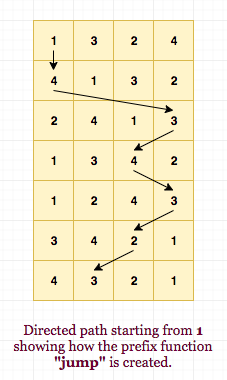
From the claim regarding Z (=X * Y), being a permuation, you can clearly see that each row is a permutation. Now consider each column as a directed path. We will now try to answer each query in O(M) complexity. Note that it is not the complete solution but a small approach towards the final one.
Consider each column the jump table. Say we want to evaluate what j (1 ≤ j ≤ m) will convert to when applying the operation from L to R. If we can do it efficiently, we can find the above summation in O(M). But we can consider a different problem. Since our final array is also permutation meaning that we can reverse map each number to a unique index, we will try to find what number gets converted to a given number x. This means, instead of going the path for finding x for a starting j, we try to find j in opposite direction from given x. Let us see how our prefix calculation for jump is helpful here.
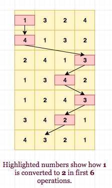
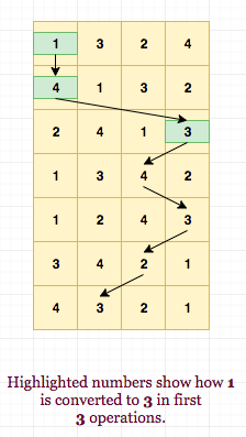
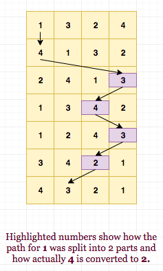
We use idea similar to prefix summation, where we calculate range sum by using prefix values for L \text{or} (L-1) and R. The directed path for a particular j from 1 to R can be broken into 2 parts, one from 1 to L and other from L to R. So, we can find which number will j convert to after first R operations. This is simply jump[R][j]. We also find which number j will convert to after first L operations, i.e. jump[L][j]. Since arrays are permutations, we can find which number actually convert to jump[R][j] by using the reversing mapping of index on jump[L][j]. This gives us the solution of above different problem. For example: Let L = 3 and R = 6 in above matrix.
We know that applying the first R = 6 operations, 1 converts to 2, 2 to 3, 3 to 1 and 4 to 4 (Directly see jump[j][R]). Also, we know that after first L = 3 operations, 1 converts to 3, 2 to 1, 3 to 2 and 4 to 4. Using the initial matrix we can see that if the operation string from L to R instead of 1 to R, 4 would have converted to 2. This is same as finding the reverse mapping of index 3 in initial matrix, which lies at index 4. Equivalently, 1 converted to 4 in path from 1 to L and then 4 converted to 3 in path from L to R. Thus, we can easily find what j converted to x when operations are applied from L to R. The below image explains the above logic in an elaborate manner:


Now, we answer each query in O(M). Below is a small pseudo-code for it:
	def init():
		# rev store the reversing mapping of index on the i^th permutation.
		for i in [1, n]:
			for j in [1, m]:
				rev[a[i][j]] = j

		for j in [1, m]:
			jump[1][j] = a[1][j]
		for i in [2, n]:
			for j in [1, m]:
				jump[i][j] = a[i][jump[i-1][j]]

	def solve(l, r):
		ans = 0
		for j in [1, m]:
			coverted_value = jump[R][j] 			# Same as B_i in summation.
			converted_from = rev[L][jump[L][j]] 	# Same as i in summation.
			ans += converted_from * converted_to
		return ans
The above logic work fine when M is small and we can answer each query in O(M). The precomputation is O(N * M). So, the overall complexity is O(N * M + Q * M). This is enough for the first 2 subtasks but not for the full solution.
For the full solution, we use idea that min(N, M) ≤ sqrt(NM). Thus, if N is small we can precompute the answer for all possible queries, which can be O(N^2) in total. We can then answer each query in O(1). The complexity for this part will be (N * M + N^2*M + Q). The first part is the initial precomputation for jump array. The second one is the calculation for each possible query in O(M) complexity and last part is the answering of each query in O(1). So, in the above pseudo code, if we just add the lines to not calculate the answer for a query which had already appeared, we can solve the full problem.
	# pre store the answer for query (l, r)
	# If the query was not evaluated, it stores -1.
	def solve(l, r):
		if store[l][r] == -1:
			# we say query for first time.
			# Calculate answer in O(M)
			store[l][r] = m
		return store[l][r]
The overall complexity of the solution will be then O(N * M + min(N^2, Q) * M). So, there are 2 cases:
-
N^2 < Q: Here the number of possible queries is smaller. So, length of one permuation will be larger. In most cases, N < M. Since, when N is smaller than M, N^2 * M will be bounded by N * M * sqrt(NM). The complexity will be O(N * M + N^2 * M) ~ O(N * M * sqrt(NM)).
-
Q < N^2. Here the number of possible queries is smaller. So, the length of one permuation will be smaller. IN most case M < N. Again the complexity will be O(N * M + Q * M) ~ O(N * M + Q * sqrt(NM)).
The space complexity of the above approach will be O(N * M + PRE), where PRE depends on the size you store for the precalulated array store.
For more details, you can refer to the editorialist’s solution for help.
Feel free to share your approach, if it was somewhat different.
Time Complexity
O(N * M + min(Q, N^2) * M) per test case.
Space Complexity
O(N * M + Q)

