Problem Link
Author: Ivan Safonov
Tester: Hasan Jaddouh
Editorialist: Bhuvnesh Jain
Difficulty
HARD
Prerequisites
DSU, Segment Trees, Dynamic Programming
Problem
You are given a grid of dimensions N * M. You are given Q rectangles on the grid with corners as (r1, c1) and (r2, c2). You can move from a point (x1, y1) to (x2, y2) inside a rectangle if x2 > x1 and y2 > y1. You are required to find the path of largest length in the grid and also the number of ways to achieve it.
Explanation
Problems related to finding largest path in grid generally relate to dynamic programming or graph traversal based solutions. Since, we also need to find the numbers of ways to achieve the number of ways to get the longest path, we will use dynamic programming approach to solve the problem.
Note: The editorial has used 0-based indexing to keep it consistent with author’s solution
Let us denote dp[i][j] as the longest path which ends at the cell (i, j). Instead of maintaining a single value for dp table, we also maintain the number of ways to achieve it. Once, the dp table is built, we just iterate through all possible maximum path lengths ending at every cell and find the maximum of all possible values. The number of ways is simply the sum of the number of ways calculated at each cell where the maximum is attained.
To consider the transitions in dp table, the naivest approach is to first store all possible transitions and then iterate over them. The complexity of this approach will be O(Q * N^2 * M^2 + N * M) which is enough to pass subtask 1. You can refer to setter’s solution below for help.
Let us first understand how to capture the transitions in a more efficient way as it will give us insights into how we deal with the rectangles and what information we store from them. The below diagram shows the set of transitions for a particular cell.
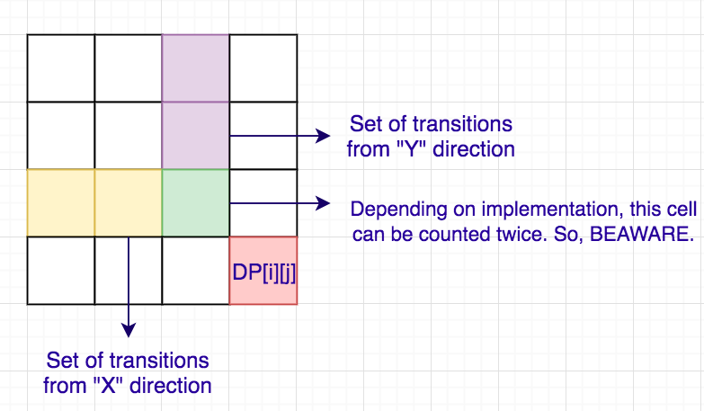
This suggest us that we need to store the X and Y coordinate till where we can move for every cell. For every cell, we can move till minimum of (x1+1) and (y1+1) among all rectangles which cover this cell. A small pseudo-code for the above logic is:
    # Assume all calculations for way_of_ways are done modulo (10^9+7)
    for i in [0, n-1]:
        for j in [0, m-1]:
           up[i][j] = i
           left[i][j] = j
    for i in [1, q]:
        x1, y1, x2, y2 = query[i]
        for x in [x1+1, x2]:
           for y in [y1+1, y2]:
               up[i][j] = min(up[i][j], x1)
               left[i][j] = min(left[i][j], y1)
    ans = 0
    for path in [0, n + m  - 2]:    # iterate over path length
        for i in [0, min(s, n - 1)]:    # iterate over row
            j = s - i   # find column based on path_length and row
            if j < 0 or j >= m:
                continue
            dp[i][j] = {1, 1}   # {path_length, num_of_ways}

            for x in [up[i][j], i - 1]:
                if dp[x][j-1].first + 1 > dp[i][j].first:
                    dp[i][j] = {dp[x][j-1].first + 1, dp[x][j-1].second}
                else if dp[x][j-1].first + 1 == dp[i][j].first:
                    dp[i][j].second += dp[x][j-1].second

            for y in [left[i][j], j - 1]:
                if dp[i-1][y].first + 1 > dp[i][j].first:
                    dp[i][j] = {dp[i-1][y].first + 1, dp[i-1][y].second}
                else if dp[i-1][y].first + 1 == dp[i][j].first:
                    dp[i][j].second += dp[i-1][y].second

            if up[i][j] < i and left[i][j] < j:
                # Avoid double counting
                if dp[i-1][j-1].first + 1 == dp[i][j].first:
                    dp[i][j].second -= dp[i-1][j-1].second
            ans = max(ans, dp[i][j].first)

    ways = 0
    for i in [0, n-1]:
        for j in [0, m-1]:
            if dp[i][j].first == ans:
                ways += dp[i][j].second

    print ans, ways
The complexity of the above pseudo-code is O(N * M + Q * N * M + N * M * (N + M)) which is enough to pass the first 2 subtasks. You can refer to author’s implementation for more details.
There are now 2 parts with us to optimise:
- Find an efficient algorithm to find the left and up values for each cells based on the rectangles in the queries.
- Optimise the calculation for dp table.
Let us first deal with the first problem. For this, we will use DSU. I will illustrate the algorithm for left array and up array calculation will be similar. Before, proceeding forward I request you to look at author’s code side-by-side as I will base my description based on his code. We will maintain a DSU for each column and sort all the rectangles by their y1 coordinates. Now we go in increasing order of y1 and update the value of left[i][j] if it was not updated. While updating the values, we also merge the rows which have the same value. The DSU has 3 values: parent of the cell, rank (size based DSU) of the cell and next row to jump to (i.e. one which might have to update by setting its left[i][j] to y1). If while considering any rectangle, left[i][j] was already set and it was updated for all rows in the column, we directly skip that column and proceed to the next one. This way, we set the left[i][j] value for each cell only once. The complexity of this part of the algorithm is therefore O(N * M * DSU + Q) ~ O(N * M + Q). Below is a diagram illustrating the process for 6 X 6 grid having 2 rectangles.
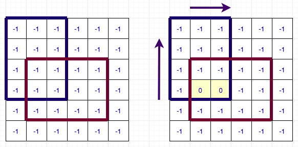
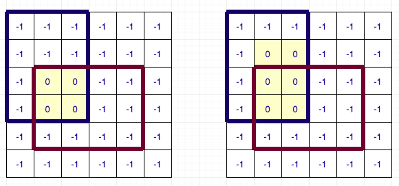
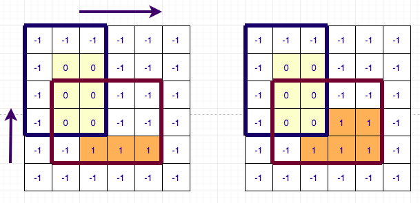
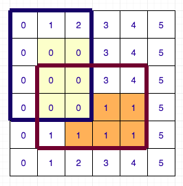
So, the only part left to optimise now is the dp calculation. Again, I ask you to refer to author’s solution for implementation details as the logic explained is completely based on it. In the above pseudo-code the only time consuming part is iterating over all possible transitions to calculate the dp value. We are iterating over all the cells in increasing order of (i + j), i.e. in increasing order of path length. Instead of iterating over the all possible transitions, we maintain a queue for each row and column. Following are the details of the queue:
- The queue is able to maintain the maximum values along with number of ways to achieve it.
- Whenever a new value if added , we remove all unnecessary items from the queue whose values is less than the current value to be inserted. If we find items with similar value, we update the number of ways.
- While deleting the element from the queue, we check if the first item in the queue has the same value as the one to be deleted or not. If yes, we proceed with deletion else we know that the item was already deleted (during the insertion process to always maintain the bigger items in the queue) and we skip the deletion. During deletion, we might also need to update the number of ways as well.
The advantage of above queue is that each element will be inserted and deleted only once in the queue and it also helps us to maintain the running maximum as well as number of ways to achieve it. Though, any insertion or deletion step can take upto O(N) steps, the complexity over all insertions and deletions will be amortised O(1). (If you are not aware about amortised complexity analysis, you can refer to this blog)
Using the above queue structure, we can easily see that each cell would be added only once and deleted only once while calculating the running maximum for every column and row. Thus, we can optimise our dp calculation to O(N * M) and solve the problem.
For more details, you can refer to the author’s solution for help.
Feel free to share your approach, if it was somewhat different.
Time Complexity
O(N * M * DSU + Q + N * M) per test case.
Space Complexity
O(N * M + Q)
Solution Links
Setter’s solution for Subtask 1
Setter’s solution for Subtask 2