Hello @all,
As I have mentioned on several posts here on forums, I am only now starting to learn graphs in a more educated, methodical and serious way, so, after I have studied DFS for few days and due to me not finding anything useful online, I decided I would write this tutorial so people can benefit from it and hopefully having an easier time in learning about graphs ![]() [note: I still don’t know much things about graphs, but, I believe that writing about a topic we learnt, it’s the best way to strengthen our knowledge on it, so, if any flaws are found, please feel free to correct them :)]
[note: I still don’t know much things about graphs, but, I believe that writing about a topic we learnt, it’s the best way to strengthen our knowledge on it, so, if any flaws are found, please feel free to correct them :)]
- Foreword and my personal view about Graphs and Graph problems in competitive programming
Graphs are everywhere! From social networks, to route planning and map analysis, passing by party planning, electric circuits analysis and even Galatik football tournaments (![]() ) there are actually few domains of Science and everyday life where Graphs can’t be seen as useful. As such, it can be quite an intimidating topic, especially because all the mathematical theory that lies behind them, seems to be a bit far from this reality.
) there are actually few domains of Science and everyday life where Graphs can’t be seen as useful. As such, it can be quite an intimidating topic, especially because all the mathematical theory that lies behind them, seems to be a bit far from this reality.
I will try to define a Graph, state some terminology and end with the first of two graph traversal methods, which, as we will see ahead, are both essential in “reading” the graph (in the sense of gathering information about its structure) and, with some additions, allows us to solve some simple problems.
- Definition of Graph and schemes of internal representation to allow easy computational analysis
Formally, we define a graph as being composed by two sets, V and E, respectively denoting the set of vertices and the set of edges. We say that vertices are connected by edges, so an edge connects two vertices together. If we generically denote a graph as G, we usually denote it by its two sets, such that the following notation is very common:
G(V, E) - is the graph G composed by V vertices and E edges.
Below is a simple example of what a graph looks like (the description is in portuguese, but, it should be easy to understand):
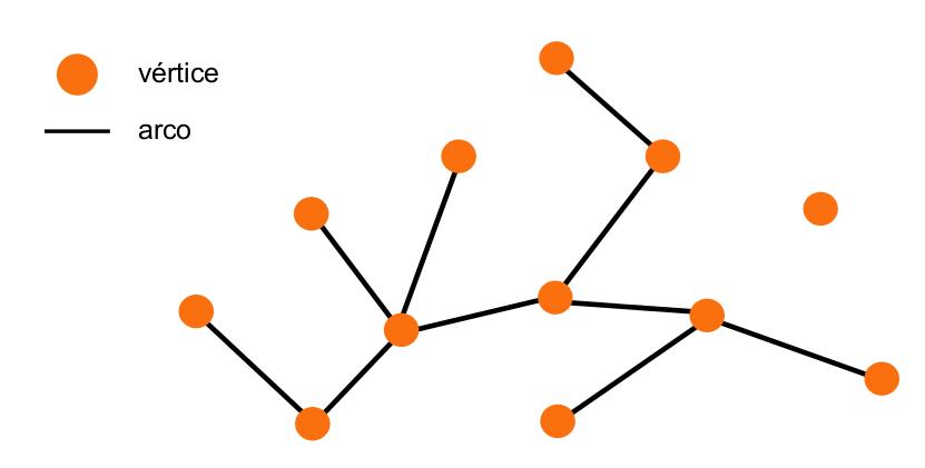
So we can immediately see that the small orange circles represent vertices and the black lines represent edges.
Please note that while it might seem a bit formal and confusing at the beginning, when we talk about graphs, this is the terminology we are going to use, as it is the only terminology we have which allows us to understand all graph algorithms and to actually talk about graphs, so, for someone who finds this a bit confusing, please twist your mind a bit ![]()
So, now we know how to define a graph and how it is formally represented. This is very important for the remaining of this post, so, make sure you understand this well ![]()
However, for sure that graphs aren’t only about defining a set of vertices and edges, are they?
Well, it turns out that things can get a little bit more complicated and there are some special types of graphs besides the generic one, which was the one we just looked at. So, let us see what more kinds of graphs we can have.
- Special types of graphs
As it was mentioned on the foreword, graphs are used to model a lot of different everyday and science problems, so, it was necessary to devise more particular types of graphs to suit such vast problem-set. Let’s see some definitions about these “special” graphs and examples of application domains:
Type 1: Directed Graph
On a Directed Graph, the edges can have an associated direction.
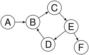
This type of graph can be particularly useful if we are modelling for example some given system of roads and/or highways to study traffic, as we can have a defined way on a given road. Making the edges directed embeds this property on the graph.
Type 2: Directed Acyclic Graph
It is alike the graph above, except that on this particular type of graph we can’t have “loops”, i.e., we can’t start a given path along the graph starting on vertex A and ending of vertex A again.
Type 3: Weighted Graph
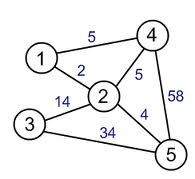
In a weighted graph, the main characteristic is that the edges can have an associated “cost”.
Mathematically speaking (and also in Operations Research) this “cost”, need not to be money. It can model any given quantity we desire and it is always “attached” to the problem we are modelling: if we are analysing a map it can represent the cost of a given road due to a toll that’s placed there, or distances between cities.
In Sports, it can represent the time taken by a professional paddling team to travel between two checkpoints, etc, etc… The possibilites are endless.
Besides these types there are also many other types of graphs (a tree, for instance, can be seen as a particular type of graph) that were devised for more advanced applications and that I really don’t know much about yet, so these will be all the types of graphs I will talk about on this introductory post.
- Representing a graph so we can manipulate it in a computer problem
It turns out that one of the hardest things about graphs for me (besides wrapping your head around the enormous amount of applications they have) is that literally everything on them is highly dependent on the problem they are modelling, even the way we decide to represent them is.
However, there are not that many ways to represent a graph internally in computer memory and even from that small universe we are going to focus solely on two representation schemes.
Representation via adjacency lists and representation via adjacency matrix.
For a better understanding, let us consider the graph below:
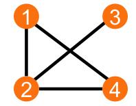
We can see now, thanks to our formal definition given earlier on this text, that this graph is composed from two sets, the set of the vertices and the set of the edges.
We have 4 vertices and 4 edges.
However, only the information concerning the number of vertices and edges is not sufficient for us to describe a given graph, because, as you might have figured out by now, the edges could be placed differently (like in a square, for example.) and we wouldn’t be able to know it.
This is why there are representations of graphs which allows us to “visualize” the graph in all of its structure, from which the adjacency matrix will be the one we will study in the first place.
- Adjacency Matrix
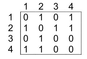
The adjacency matrix (let’s call it A) is very simple to understand and, as the name itself says, it’s a representation that is based on a matrix of dimensions V x V, where it’s elements are as follows:
A(i,j) → 1, if there exists an edge between vertex i and vertex j;
A(i,j) → 0, otherwise;
So, for the above graph, its adjacency matrix representation is as follows:
- Adjacency List
The representation as an adjacency list is usually more convenient to represent a graph internally as it allows for an easier implementation of graph traversal methods, and it is based, also, as the name states, in having a “list of lists” for each vertex, that states the vertices to which a given vertex is connected.
As a picture is worth a thousand words, here is the adjacency list representation of the above graph:
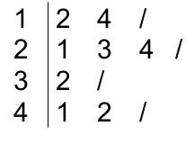
here, the symbol / is used to denote end of list ![]()
Now that we have looked into two of the most common ways of representing a graph, we are ready to study the first of two traversal algorithms, Depth-First Search.
- Understanding Depth-First Search
Depth-First search, often known as DFS (it stands for the beginning letters of each word) is a graph traversal algorithm where the vertices of the graph are explored in depth first order, with the search algorithm backtracking whenever it has reached the end of the search space, visiting the remaining vertices as it tracks back.
This idea is illustrated on the figure below where the order by which vertices are visited is described as a number (note that this is a tree, but, also, as discussed earlier, a tree is a particular kind of graph, and it has the advantage of being easy to visualize).
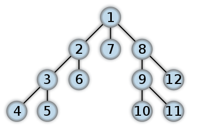
As the vertices are first explored to a certain order and then we must backtrack to explore remaining vertices, the DFS algorithm can be naturally implemented in a recursive fashion. Also please note that we assume here that the visited vertices are visited only once, so we can have, in pseudo-code:
dfs(v):
    visited(v)=true
    for i = graph.begin() to graph.end()
        if(visited(i)=false)
            dfs(i)
It’s now important to mention two things:
The first one is that in Graph Theory, DFS is usually presented in an even more formal fashion, mentioning colors and discovery times and end times for each vertex. Well, from what I understood, in programming contests the above routine is enough and the purpose of having array visited() is precisely to “replace” the color attributes that are related to discovery and end times, which I chose to ommit to keep this post in the ambit of programming competitions.
Finally, to end this explanation, what is more important to mention is that DFS usually is implemented with something more besides only that code.
Usually we “add” to DFS something “useful” that serves the purpose of the problem we are solving and that might or might not be related to two of most well known applications of DFS, which are:
- DFS applications
- Wrapping it all together: Solving FIRESC problem using what we know
FIRESC problem is the perfect problem for us to put our skills to test ![]()
Once we understand how to model the problem in terms of graphs, implemeting it is simply using one of the applications of DFS (finding connected components).
Simply, we can model this is terms of graphs as follows:
Let us define a graph whose vertices are people. An undirected edge connects two people who are friends.
On this graph, two vertices will be of the same color if they share an edge. This represents that the two people should have to go in the same fire escape route. We wish to maximize the number of colors used.
All the vertices in a connected component in this graph will have to be in the same color.
So as you see, we need to count the size of all connected components to obtain part of our answer, and below I leave my commented implementation of this problem, largely based on the work of @anton_lunyov and on the post found on this site (yes, I had to use google translate ![]() ).
).
#include <iostream>
#include <stdio.h>
#include <vector>
#include <iterator>
using namespace std;

vector<bool> visited; //this vector will mark visited components
vector<vector<int> > graph; //this will store the graph represented internally as an adjacency list
//this is because the adjacency list representation is the most suited to use DFS procedure on a given graph

int sz_connect_comp = 0; //this will store the size of current connected component (problem-specific feature)

void dfs(int v)
{
	sz_connect_comp++; //"useful feature" performed on this DFS, this can vary from problem to problem
	visited[v] = true;

	for(vector<int>::iterator it = graph[v].begin(); it != graph[v].end(); it++)
	{
		if(! visited[*it]) //note that *it represents the adjacent vertex itself
		{
			dfs(*it);
		}
	}
}

int main()
{
	int t;
	cin >> t;
	while(t--)
	{
		int n,m;
		cin >> n >> m;
		graph = vector<vector<int> > (n); //initialization of the graph
		for(int i = 0; i < m; i++)
		{
			int u,v;
			cin >> u >> v;
			u--;
			v--;
			//these are added this way due to the friendship relation being mutual
			graph[u].push_back(v);
			graph[v].push_back(u);
		}
		int res = 0; // the number of fire escape routes
		int ways = 1; // the number of ways to choose drill captains
		visited = vector<bool> (n, 0); // initially mark all vertices as unvisited
		for(int u = 0; u < n; u++)
		{
			//if the vertex was visited we skip it.
			if(visited[u]==true)
				continue;
			// if vertex was not visited it starts a new component
			res++; // so we increase res
			sz_connect_comp = 0; // init sz_connect_comp
			dfs(u); // and calculate it through the dfs, marking visited vertices
			// we multiply ways by sz_connect_comp modulo 1000000007
			ways = (long long)sz_connect_comp * ways % 1000000007;
		}
		printf("%d %d\n", res, ways);

	}
	return 0;
}
I hope you have enjoyed this short introduction to graphs and I really hope this can help anyone willing to study graphs to come across a rigorous, yet simple and understandable text ![]()
Best regards,
Bruno

