PROBLEM LINK:
Author: Devendra Aggarwal
Tester: Kevin Atienza
Editorialist: Kevin Atienza
DIFFICULTY:
Medium-hard
PREREQUISITES:
Rooted trees, dynamic programming
PROBLEM:
You are given a tree where nodes are assigned distinct values. A weird path is a path where the values increase and decrease alternately.
You are given Q queries. For each query (r,s) you need to find the sum of all weird paths in the subtree rooted at s with respect to r being the root of the original tree. Paths must contain at least two nodes.
Output all answers modulo M.
QUICK EXPLANATION:
Group the queries (r,s) according to r.
Root the tree at some node, say node 1. For each node i, compute the following values corresponding to the subtree rooted at i:
- The sum of all weird paths whose endpoints belong to different subtrees.
- The sum of all weird paths whose endpoints belong to the same subtree.
- The number of weird paths where one of the endpoints is i, and the value at i is higher than the next one.
- The sum of all weird paths where one of the endpoints is i, and the value at i is higher than the next one.
- The number of weird paths where one of the endpoints is i, and the value at i is lower than the next one.
- The sum of all weird paths where one of the endpoints is i, and the value at i is lower than the next one.
These values can be computed in linear time for all nodes with a single pass of the tree. Also, we can now answer queries (r,s) where r = 1.
Now, for the other queries. Perform another pass in the tree, so that each node becomes a root at some point. Note that whenever a new node becomes a root, the six values above must be updated in constant time. Also, when a particular node r becomes a root, immediately answer all queries (r,s) corresponding to that root.
EXPLANATION:
Let’s first answer a particular query (r,s). To do this, we must first root our tree at r.
Now, there are many kinds of weird paths. We can classify them into three types, for any given node i and the subtree rooted at i:
- weird paths where one of the endpoints is the root i. Let’s call such paths root paths.
- weird paths whose endpoints belong to different subtrees. Let’s call such paths through paths.
- weird paths whose endpoints belong to the same subtree. Let’s call such paths under paths.
Let’s understand these different types of paths. Take a look at the following tree:
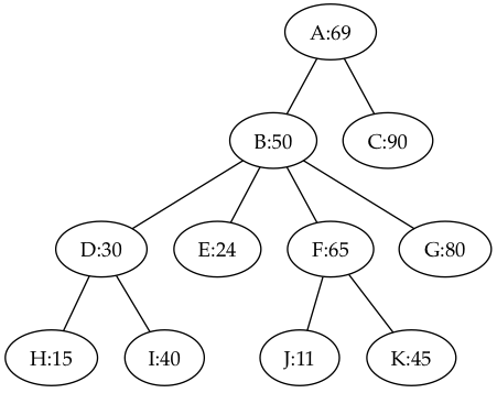
Consider the node B.
- Some examples of root paths at B are: B-E, B-J, B-K, and B-I. Note that B-H is not a root path because the values don’t alternately increase then decrease.
- Some examples of through paths at B are: D-E, I-E, and J-G.
- Some examples of under paths at B are: D-I and J-K. Note that all these paths (and the previous examples) are also under paths at A.
To answer the query (r,s), it’s natural to store the sums of these paths in each node after rooting the tree at r. But to do so, we must be able to compute them for every node i recursively after computing them for all subtrees.
Root paths
First, let’s compute the sums of all root paths. Such a path starts at i, and the remaining part of the path forms a root path at one of the subtrees of i. However, it isn’t just any root path from any subtree! This root path must still be a root path even when node i is appended to it. To compute the sum correctly, we must further classify root paths at i into two types (and we’ll sum these types separately):
- root paths where the value at i is higher than the next one. Let’s call such paths high root paths.
- root paths where the value at i is lower than the next one. Let’s call such paths low root paths.
Now, a high root path at i is simply i plus a low root path at a child whose value is lower than that of i. Similarly, a low root path at i is i plus a high root path at a child whose value is higher than that of i.
How do we calculate the sums of all high root paths at i? As described above, we simply get all low root paths at all children with values lower than that of i, and append i at each of them. But to do so, we must also know the counts of these paths!
More specifically, let’s denote by s_H(i) and s_L(i) the sum of all high and low root paths at i, and c_H(i) and c_L(i) be the counts. Then:
Let’s figure out what this means.
Let’s fix a child j with value less than that of i (i.e. \text{val} _ {j} < \text{val} _ {i}). Now, (c_L(j)+1) is the number of high root paths at i whose next node is j. The “+1” appears because we need to count the length-two path: i-j. Thus, \text{val} _ {i} must be added at least (c_L(j)+1) times in the sum, hence \text{val} _ {i}\cdot (c_L(j)+1). Now, we must also add the contributions of the remaining nodes, but this is simple: s_L(j) + \text{val} _ {j}. Note that “+\text{val} _ {j}” appears because of the contribution of j from the length-two path: i-j.
Similarly, for low root paths we have:
Since we also need c_H(i) and c_L(i), these must also be calculated. But that’s even simpler:
Through paths
Now, let’s focus on through paths. Let s_T(i) be the sum of the through paths at i. Now, a through path is simply two root paths at i that belong to different subtrees, merged together. However, again they aren’t simply any two root paths. For the merged path to be valid, the two root paths must be of the same type: i.e. either both high root paths or low root paths.
Using this characterization, we can now find an expression for s_T(i). Let j_1 and j_2 be two different children of i. Then the number of through paths whose endpoints are in the subtrees j_1 and j_2 are:
This formula is similar to the ones we have for root paths. For example, let’s look at the case “\text{val} _ {j_1},\text{val} _ {j_2} < \text{val} _ {i}”. The first term is the contribution of \text{val} _ {i} in the sum, the second term is the contribution of all nodes in the subtree j_2, and the third term is the contribution of all nodes in the subtree j_1.
Thus s_T(i) is simply the sum of this value for all (unordered) pairs of children (j_1,j_2).
Under paths
Finally, let’s focus on under paths. Let s_U(i) be the sum of the under paths at i. Consider the under paths belonging to the subtree j (a child of i). These under paths come in all four different types mentioned above: high root paths, low root paths, through paths and even under paths. The sum of all these paths is s_H(j) + s_L(j) + s_T(j) + s_U(j). Thus, the sum of all under paths at i is simply:
Computing s_T(i) quickly
Notice that the formula for s_T(i) involves a double sum on (j_1,j_2). This can make computing s_T(i) very slow, especially if some node contains a lot of children. In the worst case, this runs in O(N^2).
In order to compute s_T(i) quickly, we can imagine adding each subtree one by one, and update s_T(i) by adding the number of new through paths after adding each subtree. Actually, we not only do this for s_T(i), but also for all other values: c_H(i),s_H(i),c_L(i),s_L(i) and s_U(i).
Initially, we assume that i has no subtrees, so we have s_T(i) = c_H(i) = s_H(i) = c_L(i) = s_L(i) = s_U(i) = 0. We add the subtrees one by one, and update these values along the way.
Suppose we have a new subtree j to add, and that these six values are correct prior to adding j. We now want to update them. We first update s_T(i). There are two possibilities: either \text{val} _ {j} < \text{val} _ {i} or \text{val} _ {j} > \text{val} _ {i}.
- If \text{val} _ {j} < \text{val} _ {i}, we set increment s_T(i) by s_H(i)(c_L(j)+1) + c_H(i)(s_L(j)+\text{val} _ {j}).
- If \text{val} _ {j} > \text{val} _ {i}, we set increment s_T(i) by s_L(i)(c_H(j)+1) + c_L(i)(s_H(j)+\text{val} _ {j}).
(we invite you to check that the added value is indeed the sum of the new through paths)
Finally, the values c_H(i), s_H(i), c_L(i), s_L(i) and s_U(i) can be easily updated from the formulas above we have for them.
By combining all these techniques, we can compute all the values we want with a single pass of the whole tree!
Answering queries
The above solution is only good for queries (r,s) whose root r is the root we chose in the beginning. What about the other queries?
Suppose the tree is rooted at r_1, and we want the tree to be rooted at a new root, say r_2. Suppose for simplicity that r_2 is a child of r_1. Rooting the tree at r_2 can be done by first detaching the subtree r_2 from r_1, and then attaching the tree r_1 to r_2. However, while doing so, we must keep the six values above updated. But we already know how to update the values when attaching a new subtree! What about detaching? Well, we can simply reverse the operations above. For example the following are possible implementations of attach and detach:
def attach(i,j):
    if val[j] < val[i]:
        sT[i] += sH[i] * (cL[j] + 1) + cH[i] * (sL[j] + val[j])
        sH[i] += val[i] * (cL[j] + 1) + (sL[j] + val[j])
        cH[i] += cL[j] + 1
    else:
        sT[i] += sL[i] * (cH[j] + 1) + cL[i] * (sH[j] + val[j])
        sL[i] += val[i] * (cH[j] + 1) + (sH[j] + val[j])
        cL[i] += cH[j] + 1

    sU[i] += sL[j] + sH[j] + sT[j] + sU[j]


def detach(i,j):
    sU[i] -= sL[j] + sH[j] + sT[j] + sU[j]

    if val[j] < val[i]:
        cH[i] -= cL[j] + 1
        sH[i] -= val[i] * (cL[j] + 1) + (sL[j] + val[j])
        sT[i] -= sH[i] * (cL[j] + 1) + cH[i] * (sL[j] + val[j])
    else:
        cL[i] -= cH[j] + 1
        sL[i] -= val[i] * (cH[j] + 1) + (sH[j] + val[j])
        sT[i] -= sL[i] * (cH[j] + 1) + cL[i] * (sH[j] + val[j])
(Don’t forget to reduce the results modulo M)
Using this, we now have a way to switch roots, as long as the new root is a child of the current root. But even with just this operation, we can now answer all queries with the following method:
- Perform a special pass in the tree, where each node we visit always becomes the new root. The values must be updated every time. Note that each change of root we do is always to a child of the current root, so the method above can always be used.
- When some node r becomes the root, answer all queries (r,s) corresponding to that root during that time.
When doing a single pass of the whole tree this way, each node becomes a root at some point, which means that all queries will be answered! This also means that our solution is offline, because it requires getting all queries before processing any of them.
Time Complexity:
O(N + Q)