Editorial- RCTEXSCC (Unofficial)

[akshitm16]

As requested by @dgupta0812, here is my approach for RCTEXSCC

Problem- Expected Number of SCCs

Prerequisites:

Combinatorics, Dynamic Programming, Expected Value

Understanding The Problem:

You’re given a matrix of size M \times N and you can fill the matrix with any random integer from 1 to K independently. Find the expected value of number of strongly connected components. A cell x has a directed edge to its side adjacent cell y iff value in x is greater than or equal to value in y.

Explanation:

You can observe easily that any two cells belong to the same connected component iff they have the same number and and we can move from first cell to second cell using horizontal and vertical moves such that we don’t encounter any other number in the path.

Spoiler

The above matrix has 7 connected components.

If we are given a matrix, we can easily find the number of connected components using BFS/DFS.

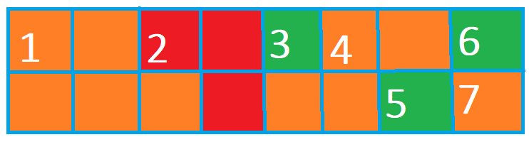
In the below explanation, color is analogous to number everywhere.

Brute Force:

Since there are are M \cdot N cells, you can create all the K^{M \cdot N} combinations and calculate the number of connected components in each combination using BFS/DFS and since each combination is equally likely, you can sum up the number of components in each combination and divide by K^{M \cdot N}. This can pass the first subtask.

Case M=1:

The matrix is an array. Let’s solve for this case

Observations

• It is easy to understand that count of matrices where the number of connected components is 1 is K because there are K choices to fill to the whole matrix with only 1 color.
• Note that the maximum number of components a matrix can have is N when every cell has a different number than its 2 (or 1 in case first or last cell) adjacent cells.
• Number of components in a matrix can range from 1 to N.

Let F(r) denote the number of matrices with r (1 \leq r \leq N) connected components.
Then our answer is simply:

\dfrac{ \displaystyle\sum\limits_{r=1}^{N} r \cdot F(r) }{K^N}

Now, the task is how to calculate F(r).

To get r components in the array, we have to make r divisions of the array. An array of size N has N-1 divider lines among which we’ve to choose r-1 to divide it into r components.

Now, in an array having r divisions, we can have K \cdot (K-1)^{r-1} choices of colors. How??

The first component has K choices. The second component has K-1 choices as we can’t fill it with same color as first. Similarly, the third component has also K-1 as we can’t fill it with color we filled in second component and so on.

Spoiler

One of the possible configurations of an array with 4 components.

So, after all this analysis:

F(r) = K \cdot (K-1)^{r-1} \cdot \binom{N-1}{r-1}

Now, plug in the value of F(r) in the above Formula to get AC in Subtask 2.

Case M=2:

Now, we have a matrix with 2 rows and N columns. Let’s tackle this case.

Let’s define dp[i][j] (1 \leq i \leq N; 1 \leq j \leq 2).

• dp[i][1] denotes total number of components possible till i^{th} column if both the cells in the i^{th} column are filled with same value. Note that this count is for a single instance out of all possible cases of equal values (which is K) in the i^{th} column.

• dp[i][2] denotes total number of components possible till i^{th} column if both the cells in the i^{th} column are filled with different values. Note that this count is for a single instance out of all possible cases of different values (which is K^2-K) in the i^{th} column.

• Clearly, total number of components we can get till i^{th} column are:

(K \cdot dp[i][1]) +((K^2-K) \cdot dp[i][2])

• Base Cases:
  dp[1][1]=1 as filling the first column with same color will give only 1 component.
  dp[1][2]=2 as filling the first column with two different colors will give 2 components.
  Total number of components we can get if there’s only 1 column: (K \cdot 1)+((K^2-K) \cdot 2)

Transitions:

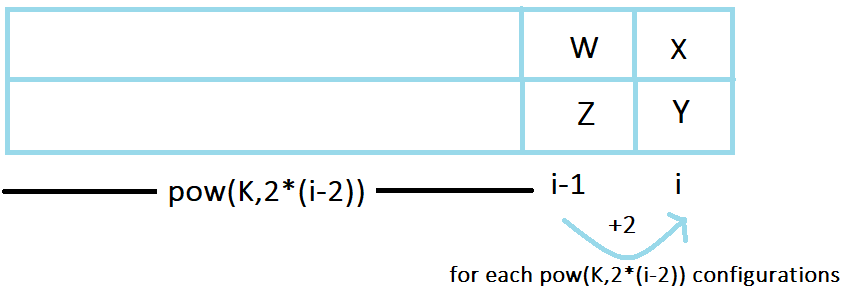
Now, the next steps might be intimidating but bear with me.

We want to calculate dp[i] from dp[i-1].

Steps to calculate dp_{i,1}

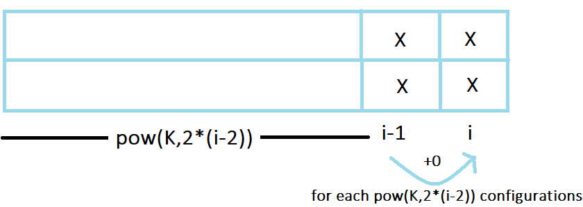
Let’s say for calculation of dp[i][1], we fill both the cells in i^{th} column with some X color. Now for {(i-1)}^{th} column, we can have K^{2} cases out of which in K cases both the cells in {(i-1)}^{th} column will be of same color and for K^2-K cases, the cells will be of different color.

Out of the K cases (of equal color), first consider the case in which {(i-1)}^{th} column has cells of color X. In this case, there will be no increase in components from i-1 to i.

Hence, dp[i][1]+=dp[i-1][1]+(0 \cdot K^{2\cdot(i-2)})

Spoiler

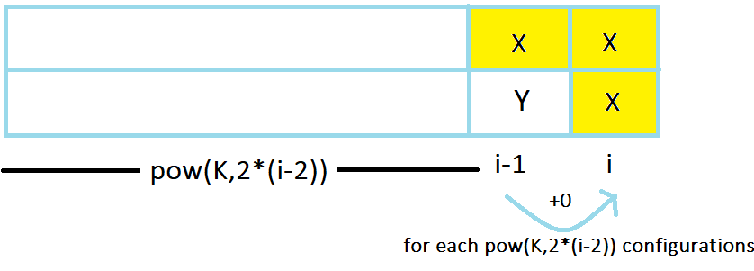
Now, out of the K cases of equal color, in K-1 cases the color X will mismatch and we’ll get increase in number of components by 1 for each of K^{2 \cdot (i-2)} possible configurations.

Hence, dp[i][1]+=(K-1) \cdot (dp[i-1][1]+(1 \cdot K^{2\cdot(i-2)}))

Spoiler

For rest K^2-K cases (of different colors), there will be 2\cdot K-2 cases when the value in the upper cell is X or value in the lower cell is X. In this case, there will be no increase in the number of components.

Hence, dp[i][1]+=(2 \cdot K-2) \cdot ( dp[i-1][2]+(0 \cdot K^{2\cdot(i-2)}))

Spoiler

For rest of the K^2-3\cdot K+2 cases of different colors, both the values will be different to X and hence we’ll get increase in number of components by 1 for each of K^{2 \cdot (i-2)} possible configurations.

Hence, dp[i][1]+=(K^2-3\cdot K+2) \cdot ( dp[i-1][2]+(1 \cdot K^{2\cdot(i-2)}))

Spoiler

Full calculations for dp_{i,1}

dp[i][1]+=dp[i-1][1]+(0 \cdot K^{2\cdot(i-2)})
dp[i][1]+=(K-1) \cdot (dp[i-1][1]+(1 \cdot K^{2\cdot(i-2)}))
dp[i][1]+=(2 \cdot K-2) \cdot ( dp[i-1][2]+(0 \cdot K^{2\cdot(i-2)}))
dp[i][1]+=(K^2-3\cdot K+2) \cdot ( dp[i-1][2]+(1 \cdot K^{2\cdot(i-2)}))

Steps to calculate dp_{i,2}

Now, for the calculation of dp[i][2], we fill upper cell in the i^{th} column with color X and lower cell with color Y. Now for {(i-1)}^{th} column, we can have K^{2} cases out of which in K cases both the cells in {(i-1)}^{th} column will be of same color and for K^2-K cases, the cells will be of different color.

Out of K cases (of equal color), there will be 2 cases when either both the colors will be X or both will be Y. In this case, the number of components will increase by 1 for each of K^{2 \cdot (i-2)} possible configurations.

Hence, dp[i][2]+=(2) \cdot ( dp[i-1][1]+(1 \cdot K^{2\cdot(i-2)}))

Spoiler

Out of K cases (of equal color), in rest of the K-2 cases, X and Y both will mismatch and hence we’ll get increase in number of components by 2 for each of K^{2 \cdot (i-2)} possible configurations.

Hence, dp[i][2]+=(K-2) \cdot ( dp[i-1][1]+(2 \cdot K^{2\cdot(i-2)}))

Spoiler

For rest K^2-K cases (of different colors), there will be 1 case when the value in the upper cell is X and value in the lower cell is Y. In this case, there will be no increase in the number of components.

Hence, dp[i][2]+=(1) \cdot ( dp[i-1][2]+(0 \cdot K^{2\cdot(i-2)}))

Spoiler

Among K^2-K cases (of different colors), there will be 2 \cdot K-4 cases when either (the first color is X and second color is some Z) or (the second color is Y and first color is some Z). In this case, the number of components will increase by 1 for each of K^{2 \cdot (i-2)} possible configurations.

Hence, dp[i][2]+=(2 \cdot K-4) \cdot ( dp[i-1][2]+(1 \cdot K^{2\cdot(i-2)}))

Spoiler

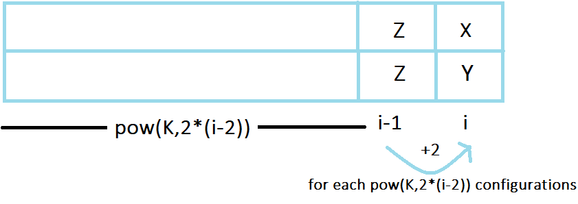
The number of cases left are (K^2-K)-(1)-(2 \cdot K-4)=(K^2-3 \cdot K +3). In these cases, both the upper cell and lower cell of i^{th} column will mismatch and the number of components will increase by 2 for each of K^{2 \cdot (i-2)} possible configurations.

Hence, dp[i][2]+=(K^2-3 \cdot K +3) \cdot ( dp[i-1][2]+(2 \cdot K^{2\cdot(i-2)}))

Spoiler

Full calculations for dp_{i,2}

dp[i][2]+=(2) \cdot ( dp[i-1][1]+(1 \cdot K^{2\cdot(i-2)}))
dp[i][2]+=(K-2) \cdot ( dp[i-1][1]+(2 \cdot K^{2\cdot(i-2)}))
dp[i][2]+=(1) \cdot ( dp[i-1][2]+(0 \cdot K^{2\cdot(i-2)}))
dp[i][2]+=(2 \cdot K-4) \cdot ( dp[i-1][2]+(1 \cdot K^{2\cdot(i-2)}))
dp[i][2]+=(K^2-3 \cdot K +3) \cdot ( dp[i-1][2]+(2 \cdot K^{2\cdot(i-2)}))

Now, our final our answer is:

\dfrac{ (K \cdot dp[n][1]) +((K^2-K) \cdot dp[n][2]) } {K^{2 \cdot N}}

Implementation:

Click

Click Again

If you find any mistakes or something is unclear, please feel free to point out.

[lemongrab]

Very nice editorial! And thanks for the images, makes the point clear in one glance.

[dgupta0812]

Awesome editorial brother !!

[cubercoder]

Thanks for this,
I actually had the same solution and was originally a bit overwhelmed when I saw the original Editorial.

[mearnest]

There is a simpler solution using linearity of expectation.

For the subtask with M=1, the number of connected components is equal to 1 plus the number of pairs of adjacent entries who have different values. Since the probability two adjacent values are different is (K-1)/K, linearity of expectation implies the answer is 1 + (N-1)\cdot (K-1)/K.

The general problem is more complicated, but can still be solved with some simple summations rather than DP. The answer is

1+(N-1)\frac{K-1}K+ \\ +\sum_{i=1}^{N-2}(N-1-i)\frac{(K-1)^{i+2}}{K^{2i+1}}\\ +2\sum_{i=1}^{N-1}(N-1-i)\frac{(K-1)^{i+1}}{K^{2i}}\\ +\frac{(K-1)^{N}}{K^{2N-1}}\\ -\sum_{i=3}^N(N-i+1)\frac{(K-1)^{i-2}}{2i-1}

The first term 1+(N-1)\frac{K-1}K accounts for connected components which include at least once cell in the bottom row; it is actually an overcount, and is corrected by the last summation. The middle three terms account for all possible connected components which exist entirely in the top row, where i represents the length of the component.

Here is a python implementation: CodeChef: Practical coding for everyone

[i_am_legend1]

Hi @akshitm16 I was trying to write dp for m=1 in a similar way you did for m=2 ,but it’s not correct

---

vector dp(n+1);
dp[1]=1;
fi(2,n+1)
{
dp[i]+=dp[i-1];
dp[i]+=(k-1)(dp[i-1]+binpow(k,2(i-2)));
}
num ans=(k*dp[n])*binpow(binpow(k,n),mod-2);
cout<<ans<<’\n’;

---

please help me in finding the mistake.

[akshitm16]

You’re multiplying i-2 with 2. That’s the only mistake I see.

[i_am_legend1]

Oh dammit .
Thanks for helping ,that was so silly of me.